Your Agent Decides at 0.8 Confidence. You Never Measured 0.8.

A team I was helping ran an agent that triaged inbound support tickets. For each ticket the model returned a category and a confidence number, and the pipeline acted on it: above 0.8 it auto routed and closed the loop, below 0.8 it went to a human. It worked in the demo. Three weeks into production, billing tickets with a cheerful 0.82 were landing in the security queue, and the on call engineer had stopped trusting the number entirely and was reading every ticket by hand. The score had not broken. It had never meant what the threshold assumed it meant.

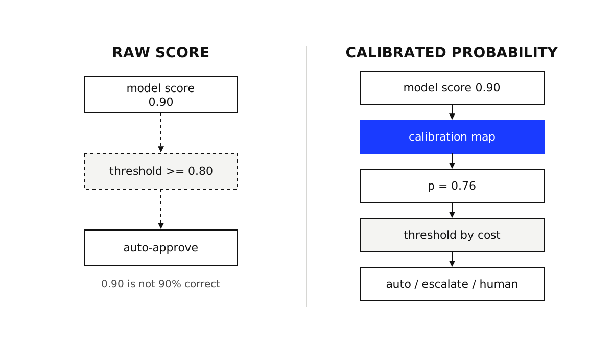
This is a different failure from a model that crashes or returns bad JSON. The decision looks successful. A number came back, it cleared the bar, an action fired. What nobody checked is whether 0.8 from this model, on this traffic, actually corresponds to being right eighty percent of the time. Almost always it does not, and the threshold you picked is sitting on a number that was never a probability.

The decision is not an answer

Most writing about LLM reliability is about answers, text a person reads. A large and growing share of what agents actually do is decisions: classify this ticket, is this refund allowed, how severe is this incident, which of these two drafts is better, route this to the cheap model or the expensive one. The output is not prose for a human to weigh. It is a number that drives an automated action, thousands of times a day, with no one in the loop to catch a bad call.

OpenAI leaned into exactly this split this month. Its Decisions API, in public beta since the sixth of October, is a dedicated endpoint for decisions rather than answers. You hand it an input and a list of questions, and it returns structured outputs in three shapes: a predicate returns the probability a condition holds, a choice picks one value from a set and reports a probability for each option, and a score rates the input against ordered levels as a probability weighted average of the level indices. The framing is the useful part, whichever vendor you use. A decision wants a probability, not a sentence.

The trap is assuming the probability is trustworthy because it arrived as a float. A number between 0 and 1 is not a probability just because it is shaped like one. It becomes a probability only when you have checked that the number tracks the frequency of being right, and that check is what almost nobody does before wiring a threshold to an action.

Why 0.9 is not 90 percent

Calibration is the property you are missing. A model is calibrated when, across all the times it says 0.9, it is correct about ninety percent of the time. Modern models are not calibrated by default, and the training process is why. The finding goes back to Guo et al. on the calibration of modern neural networks: as networks got deeper and were trained harder, their raw confidence drifted away from their accuracy, almost always toward overconfidence. Instruction tuning and RLHF push the same direction, because a confident tone reads as a better answer to a human rater, so the model learns to sound sure.

The second thing that bites is that accuracy and calibration are different axes, and the best model on one is not the best on the other. The recent ConfidenceBench study makes this concrete: the most accurate model in their evaluation is not the best calibrated one, and several models score worse than a calibrated random baseline on confidence while still posting reasonable accuracy. So you cannot reason "we use a strong model, its confidence is probably fine." Strength buys you accuracy. It does not buy you a confidence number you can threshold.

This is the same disease the LLM judge essay treats from the evaluation side, where a biased judge's score propagates into every release it gates. Here the score is driving a live action rather than a release decision, so the blast radius is your production traffic. And it is the raw material the abstention gate relies on: that essay is about whether an agent should answer a user at all, this one is about whether the confidence behind any automated decision means what your threshold assumes. Both need the same thing next, a number you have measured.

Measure it before you trust it

You do not fix calibration by arguing about it. You measure it, with labeled outcomes from your own traffic, not from the eval set you wrote at the start of the project, because production inputs drift and that drift is exactly what a living eval set built from production traces is meant to catch. Collect a few hundred decisions where you know the correct outcome. Bucket them by the confidence the model reported. In each bucket, compare the average confidence against the fraction that were actually correct. That comparison, plotted, is a reliability diagram, and a calibrated model sits on the diagonal. Summarized as a single number it is Expected Calibration Error, the traffic weighted average gap between confidence and accuracy.

import numpy as np

def expected_calibration_error(confidences, correct, n_bins=10):
    """confidences: model's reported probability per decision, 0..1
    correct: 1 if the decision was right, else 0. Returns ECE in [0,1]."""
    confidences, correct = np.asarray(confidences), np.asarray(correct)
    edges = np.linspace(0.0, 1.0, n_bins + 1)
    ece = 0.0
    for lo, hi in zip(edges[:-1], edges[1:]):
        # last bin is closed on the right so a score of exactly 1.0 lands somewhere
        in_bin = (confidences > lo) & (confidences <= hi) if hi < 1 else (confidences > lo)
        if not in_bin.any():
            continue
        avg_conf = confidences[in_bin].mean()
        accuracy = correct[in_bin].mean()
        ece += (in_bin.mean()) * abs(avg_conf - accuracy)  # weight by bucket share
    return ece

# ece below ~0.02 is tight; above ~0.1 your thresholds are built on sand.

Run that once and you usually get a number north of 0.1, which in plain terms means an answer the model called 0.9 was right closer to seventy five percent of the time. That is not a rounding error. It is the gap between the service level you think you are shipping and the one you are actually shipping, and it is invisible until you put the two numbers side by side.

Correct the score, do not just rank it

Once you can measure the gap you can close it. The cheapest fix that works is the one Guo et al. recommend: temperature scaling, a single parameter fit on a held out labeled set that rescales the scores so the reliability curve lands back on the diagonal. It does not change which decisions rank above which, so your accuracy is untouched. It only makes the number mean something. When the miscalibration is lopsided rather than a uniform overconfidence, isotonic regression fits a free form monotone mapping instead, at the cost of needing more labeled data to avoid overfitting the curve.

from sklearn.isotonic import IsotonicRegression

def fit_calibrator(dev_conf, dev_correct):
    """Fit a monotone map from raw score to observed accuracy on a labeled dev set.
    Returns a function you apply to future raw scores before thresholding."""
    iso = IsotonicRegression(out_of_bounds="clip", y_min=0.0, y_max=1.0)
    iso.fit(dev_conf, dev_correct)      # learns raw_score -> P(correct)
    return lambda raw: float(iso.predict([raw])[0])

calibrate = fit_calibrator(dev_conf, dev_correct)
# raw 0.90 from the model might map to a calibrated 0.76 you can actually act on
p = calibrate(0.90)

The important move is conceptual. You stop treating the model's output as the probability and start treating it as a raw score you pass through a calibration map you own. The map is small, it is cheap to refit, and it lives in your code where you can version it, not inside a model you do not control. That is what makes the number defensible when someone asks why a ticket got auto closed.

If your provider hides token logprobs, and many do, nothing above changes. You get the raw score from an outside signal instead, verbalized confidence or the spread across a few samples, the same signals the consensus sampling approach uses to vote out flaky steps. The calibration step is identical: map whatever raw score you have to an observed accuracy on your labeled set.

Set the threshold by what a wrong call costs

A calibrated probability is still not a decision. The decision is where you put the line, and the line is not a vibe, it is arithmetic on cost. If a false positive, auto approving something you should not have, costs you C_fp, and a false negative, sending a safe case to a human, costs you C_fn, then the break even probability above which acting is the cheaper bet is C_fp divided by the sum of the two. That is the whole rule. The reason calibration had to come first is that this arithmetic is meaningless on a raw score: you cannot weigh costs against a number that is not a probability.

def decide(p, cost_fp, cost_fn, gray=0.1):
    """p: calibrated probability the positive action is correct.
    Returns auto, escalate (ambiguous band), or human (clearly not safe)."""
    tau = cost_fp / (cost_fp + cost_fn)   # break-even threshold from costs
    if p >= tau + gray:
        return "auto"                     # clearly above break-even, act
    if p >= tau - gray:
        return "escalate"                 # near the line, spend more before acting
    return "human"                        # below break-even, hand it off

# Expensive mistake (cost_fp=20, cost_fn=1) pushes tau to ~0.95: act only when very sure.
# Cheap mistake, costly deferral (cost_fp=1, cost_fn=20) pulls tau to ~0.05: act freely.

Notice the three way outcome rather than a single cutoff. A band around the break even point is where you escalate: spend more compute, call a bigger model, or hand it to a person, exactly the move the cost aware model router and the reasoning effort budget make on easy versus hard inputs. The cost of a wrong decision, not the raw confidence, is what sets where that band sits. A refund approval and a content flag that merely queues a review do not get the same threshold, because their mistakes do not cost the same.

The parts that bite

Calibration is local, and it drifts. The map you fit on billing tickets will not hold for security tickets, and the one that held last month slips when traffic shifts, when a prompt changes, or when the provider updates the model under you. Treat the calibration map like any eval: segment it where volume justifies, store the ECE as a number you can regress, and refit on a schedule. A calibration you earned once and never rechecked is describing a model that no longer exists.

The score type matters more than it looks. A probability weighted average, the shape OpenAI's score questions return, is a useful ordered summary, but it is an expected value, not a probability, so it reads badly as a threshold input. For a true gate, prefer a predicate or a per option probability you can actually calibrate and threshold, and keep the averaged score for ranking and dashboards.

A dedicated decision endpoint does not absolve you. It hands you a cleaner raw score than scraping a number out of chat text, which is real progress, but OpenAI's own guidance is explicit that you test thresholds against labeled examples from your application and choose them by the cost of false positives versus false negatives. The vendor cannot know your costs and does not promise calibration against your traffic. The measurement is still yours to run.

Watch coverage, not just error. Push a threshold up to make the automated decisions safer and you send more work to humans, which can quietly erase the savings that justified the automation. Track the fraction you auto handle alongside the error rate on what you handled, and read them as a pair. An agent that auto decides five percent of tickets flawlessly has not solved the problem, it has renamed it.

The takeaway

A confidence number that arrives shaped like a probability is not one until you have checked it against outcomes. Models are overconfident by construction, the strongest model is not the best calibrated, and a threshold wired to a raw score is a guess wearing a decimal point. The fix is three unglamorous steps you own end to end: measure the gap with a reliability diagram and ECE on real traffic, correct the score with a small scaling map you can version and refit, and set the line by what a wrong decision costs rather than by what felt safe. A dedicated decisions endpoint gives you a better raw score to start from, and changes none of that work.

Do this and the number on the dashboard becomes a service level you can defend to the person whose refund got auto approved. Skip it and you are automating decisions on a score that reads high and never tells you which calls it got wrong. If your agent is routing, approving, or flagging on a confidence it has never calibrated, that gap is measurable in about a week. Book a consultation call and we can measure your ECE on your own traffic and set the thresholds to match what your mistakes actually cost.